Showing posts with label phased array. Show all posts

Monday, 12 May 2014

KAIRA Status Map

We have a new status map showing the situation with KAIRA.

This shows the actual current status:
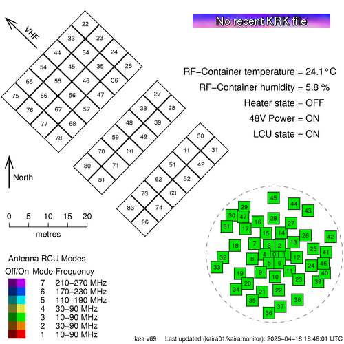


This is available from the Status page, which can be found in the title bar of this web log.

The map shows the array layout of the antennas. The High-Band Antenna (HBA) tiles are in the top left and the Low-Band Antenna (LBA) aerials are in the lower right.   The layout is to scale, which is shown, and the direction to the VHF transmitter at Tromsø, is also indicated.

The antennas are numbered and they are also colour coded to show the Receiver Unit (RCU) mode. KAIRA has 96 RCUs and the RCU mode indicates which combination of antenna plus band-pass filter is used for the processing. Sometimes the entire array is configured to a single RCU mode and at other times it is mixed with several different modes for different antennas.

If an antenna is enabled, then the colour is bright, but if it is switched off, then it is dulled down.

In the case of a plain grey antenna icon, this means the antenna is shut down, either for maintenance, or as a result of damage.

Sometimes an antenna might be shaded with two colours like a two-tone maritime-Z-pennant. This is because each antenna has two polarisations, and there will be occasions when the RCU number/status for each polarisation is not the same.

In the bottom left, there is the legend and in the top right is the status label and the current RF-container parameters.

The image at the start of this post is "live". If you update the page, you might see ti change, depending on what KAIRA is doing. But to give an indication of what the status map might look like, here are some other static examples:

A "357"-mode solar observation. The grey antennas
are those knocked out by the March 2014 blizzard.

A mode-3 riometry observation. Storm-damaged antennas
are also present in this particular example.

Monday, 23 December 2013

Manx-arrays revisited

Yes, it is Monday again and time for something a bit technical to kick us into the new working week.

A few weeks back we had a posting about the so-called "manx-array" layout for baseline distributions. Well, our colleague Björn Gustavsson (UiT) has provided today's figure. He points out another interesting fact about the manx-array, namely that it is possible to cascade it into a fractal Cantor-dust type configuration -- which gives fairly nice base-line distributions too!


Cascading manx-arrays. (Image: B. Gustavsson)


In the diagram, the antenna locations are on the left-hand graphs, and the uv-coverage (or baseline-distribution) is on the corresponding right-hand side graph.

Exercise for the reader... are there any redundant arrays? And, is there a cascade ratio that is optimal for an infinite distribution?

Monday, 9 December 2013

Six-element non-redundant array

We've been discussing array layouts recently, with regard to riometry and outlines for LOFAR superstations. There are lots of possibilities of course, but there is one which is rather elegant as well as being practical. Today, we are featuring it here.

The imaging or beamforming properties of an array of antennas is related to the baselines that the array possesses. A baseline is the vector between any two antennas in the array. If an array has 3 antennas, it will have 3 baselines: the baseline between antennas 1 and 2, between 2 and 3 and between 3 and 1. A 4-antenna array will have 6 baselines, a 5-antennas array will have 10 and so on. The number of baselines is related to the number of antennas N by the expression B = N (N-1) / 2.

Although more antennas means more baselines, these baselines may not necessarily be unique. For example, let's imagine 3 antennas, equi-spaced on a line. The baseline from 1 to 2 will be exactly the same as the baseline from 2 to 3. These are referred to as redundant baselines. Although the extra antennas add sensitivity, the fact that the baselines are identical mean they do not add to the imagine quality (i.e. the beampattern).

Finding an array layout with no redundant baselines can be tricky. Even harder, is finding one whose baselines are neatly distributed, thus sampling as much of the baseline parameter space as possible. This parameter space is typically plotted on a graph referred to as a uv-diagram (the differential spatial axes are u and v).

However, there is one which actually has a uniform distribution for a relatively small number of antennas. It is the next logical extension of the 3-antenna equilateral array. The layout of the antennas looks like this:

A manx-array antenna layout (Image: D. McKay-Bukowski)

In the diagram the antenna positions are labelled as 0, 1, ... 5. The antennas themselves are not necessarily hexagonal, but it does fit nicely on a hexagonal grid, thus making it easy to visualise. The baselines for this grid look like this:

The uv-coverage of a manx array (Image: D. McKay-Bukowski)

In the uv-diagram, the baselines are labelled XY, where XY is the baseline for Antenna X - Antenna Y. As you can see, the baselines are equispaced with no redundancies.

I was introduced to this array by Björn Gustavsson (UiT), but I don't have a reference for who came up with it originally. We tend to refer to it as a Manx Array, owing to the similarity between the antenna layout and the triskelion that appears on the brattagh Vannin (the flag of the Isle of Man). But if anyone has any original references, please let us know!


PS:  It is delightful to work with hexagonal grids. It takes me back to the old days of playing with hexgrid-based games.

Monday, 6 August 2012

Triple-A: Aperture Arrays at ASTRON


There's a new weblog specifically for aperture arrays in radio astronomy, written by Ilse van Bemmel.


Although KAIRA has a much bigger scope that just astronomy, this new feature might well be of interest to many of our readers. We asked Ilse for an introduction, and this is what she sent us:

When you think about radio astronomy, most people imagine the fantastic big dishes that collect the radio emission from the farthest regions of the Universe. However, to see the faintest possible structures, a very large number of dishes is needed, and this rapidly becomes very expensive. A new technology to make very cheap and flexible radio telescopes is aperture arrays. These are in essence large collections of fairly simple and cheap receivers, which are combined with a computer to mimic a single large dish.
This technology was developed for radio astronomy at ASTRON over the last decades, and is now at a level at which it can be used to build radio telescopes. The first one of this kind is the LOFAR (www.lofar.org) telescope, currently the world's largest radio observatory. However, LOFAR is still small compared to the ultimate goal: the Square Kilometre Array (SKA, www.skatelescope.org).
For low frequencies there is no doubt that aperture arrays are the best technology for the SKA. But for the 'classical' radio astronomy frequencies around 1GHz, aperture arrays have to compete with the well-known and well-understood dishes. Aperture arrays are cheaper, can look in multiple directions at once, can observe over enormous frequency ranges, and can be triggered to look at a particular source pretty much instantaneous. However, they are the new kid on the block, and processing the data into scientifically sensible images is still a challenge.
In this blog I describe my efforts at understanding how aperture arrays work from an astronomical perspective, and my attempts to engage fellow astronomers to embrace the technology (pun towards EMBRACE fully intended). Follow me through the circle which engages engineers ('do you have an exact number for it?'), discussions with fellow astronomers ('within an order of magnitude is fine...'), and the management ('there is currently no budget for that').

It's a great web log and is recommended to all who are interested in the progress being made in radio astronomical phased arrays.


Thursday, 28 April 2011

How do KAIRA and LOFAR work? — Part 11 : Ambiguities

As we’ve seen over the past few instalments of this series, as the direction in which the radio waves approach the telescope changes, the received signals will go out of phase. This effect reduces the sensitivity of the telescope in that particular direction. Additionally, by adding a delay to the electrical signals (whether the analogue electrical signals or the digitised version) the direction in which the telescope is sensitive can be moved.

But there is a problem.

As the incoming direction changes, the signals go out of phase, and thus cancel. However, if the direction continues to change, the signals can actually start to come back in phase again. The peak of one wavefront signal comes through one receiver and adds together with the peak of a different wavefront signal that has come through the other receiver. Click on the following image to get a full-sized version and you'll see what we mean.


At first appearance this might seem like a good thing, as the telescope seems to be sensitive to several directions at once. But it is not. Instead, this leads to an ambiguity. If a signal is received, it is impossible to tell whether that source of that signal is at the ‘on axis’ direction of the telescope, or is in a region off to one side.

These directions of sensitivity that are not in the intended pointing direction of the array are referred to as ‘sidelobes’.

However, there is a way to alleviate this. This is done by adding more receivers to the array. In our example, let’s consider adding a 3rd receiver between the original two. Now, even though there may be ambiguity on the signals received by the first two receivers, the middle receiver is out of phase with the others.

The addition of additional receiving elements helps reduce the sensitivity of some of the unintended directions. This effect is sometimes referred to as ‘suppressing the sidelobes’. If we were to sketch a graph showing an approximation of the sensitivity of the system to a particular direction as we look at angles to the left and right of the primary pointing direction, it would look something like this:
Adding more and more receivers improves this even further. As more receivers are added, it will have the effect of suppressing more of the sidelobes and thus reduce the ambiguity of the telescope.

Tuesday, 26 April 2011

How do KAIRA and LOFAR work? — Part 10 : Multi-beam operations

As we saw in the last web log entry in this series, digitising the signals gives some distinct benefits when it comes to adding a delay. Apart from being able to do it very precisely, you can change it quickly. However, digital data has another massive advantage.

It can be easily copied.

So, if you make a copy of your digital data, you can process each copy however you want. If you want to filter it differently (for example, to ‘listen’ at a different frequency) you can. However, you can also make a copy and apply different sets of delays to it. This means that if one copy of the data has one set of delays and another copy has a different set for the different antennas involved, then these two copies will be sensitive to different directions.

In other words the telescope will be looking in two different directions at once!

This technique of introducing delays and combining the signals to change the direction in which the telescope is sensitive is known as ‘beamforming’. And making digital copies and delaying them differently to sensitive in several directions is called ‘multiple beamforming’ (or sometimes ‘forming multiple beams’).


In the above diagram (which you can click to see a larger version), each received signal is digitised and split into two copies. The copies are fed into the different digital delay units (D1, D2, D3 & D4). Let’s say that D1 and D3 have no delay at all. The added signal from these will be sensitive to something from directly overhead. In this case, the original radio signal was coming in obliquely; it adds out-of-phase and no output is seen. On the other hand, by adding a delay to D2 (but not D4), the added signal from these will be sensitive to the oblique radio wave. It adds in phase and a strong output is seen.

Because the data is digital, you can copy and delay it as much as you want and there is no degradation of the signal. If you want to be sensitive in more directions, simply add more copies, delay units and adders. The limits are not related to the signal, but rather to issues of equipment, memory, power, space (... and ultimately the project budget).

In practice, systems like KAIRA and LOFAR are also limited by the amount of digital signal processing equipment. At the time of writing this, LOFAR is routinely operating with up to 30 or so different beams. However, some experimental observations have been carried out with over 250 beams.

Wednesday, 6 April 2011

How do KAIRA and LOFAR work? — Part 9 : Digital beam steering

As we saw in the last web log post on how it all works, we can adjust the cable length and thus the delay in the electrical signal to determine which directions will add in-phase (and thus be stronger) and which will add out-of-phase (and hence cancel each other out).

Although this is sometimes done by adding more cable, it doesn’t have to be. The only thing that is important is that there is the correct delay.

So, instead of using cable, we can digitise the signal and then save the data, wait a little while, and only then load them back again to feed into the adding electronics.If you are constantly taking digital data and storing them, then it is exactly the same as writing numbers into sequential memory. And if you are reading them back out at a fixed delay, then it is the effectively same thing: reading numbers from sequential memory.

As long as those data are always being written into the memory at a nice fixed rate, and are being read back out again at the same rate, all you need to do is adjust the offset between the write position and the read position and you are controlling the delay.

The limitations are that the accuracy at which you represent the incoming wave is a function of the speed at which it is being sampled. Fast memory and fast sampling requires some sophisticated electronics. There is also a limitation that the total amount of delay you can add is a function of the speed at which you are writing/reading and the total amount of memory you have.

However, with modern digital electronics, this sort of memory is relatively cheap. Additionally, changing that write-read offset (and thus the delay) can be done very quickly. As a result, you can change the signal delays, and hence the pointing direction of the entire array very quickly. To go from one side of the sky to the other takes something in the order of a millisecond.

Try doing that with a 100m radio dish!

Alternatively, you can gradually adjust the delay and move the sensitivity of the array quite slowly. This is ideal for tracking celestial sources as they appear to move slowly across the sky due to the Earth’s rotation.

However, despite the power of digital signal processing on changing the directional sensitivity of the phased array, there is another benefit as well. Stay tuned!

Monday, 4 April 2011

How do KAIRA and LOFAR work? — Part 8 : Steering a phased array

Last time, we saw that a couple of detectors can be used to collect signals and that because they will add in phase from some directions and not others, there is a certain directionality to the system.

In principle, you can ‘steer’ this system to look in different directions by tipping it, but that’s not particularly efficient. The real advantage is that without moving the antennas you can change the directionality of the overall system by changing the lengths of the cables.

Let’s consider the off-zenith case from the last part.

If we now add a bit of extra cable, these off-zenith signals now add in-phase again.

In fact, the zenith signals are the ones now out of phase when they are combined electrically. So, by adding some cable length, you can control the direction in which the array is sensitive. That is, you can steer its ‘looking direction’ around the sky without actually moving the antennas themselves.

Some phased arrays indeed use cables to adjust their pointing direction. The VHF radar in Tromsø is one such system. It is mechanically steered in the vertical direction and horizontally pointed with a phased array. By manually changing the cables, the horizontal pointing direction of the array can be altered by 15 degrees.

A view inside the feeder bridge of the VHF system
at Tromsø. (Photo courtesy Mike Rietveld)


Because this needs to be done by hand, it is not patch the cables that quickly, so these sorts of directional changes are not done too often.

Although still useful (rotating a 120×40m antenna in azimuth is tricky!) there is another technique which has recently become affordable and which makes arrays like KAIRA, LOFAR and the SKA practical.

Thursday, 31 March 2011

How do KAIRA and LOFAR work? — Part 7 : Phased arrays

Finally, we're onto the phased arrays!

The phased array concept is central to the LOFAR project. Phased arrays were developed by the German physicist Karl Ferdinand Braun in 1905. During the Second World War, they were used for radars, first by the Luftwaffe and then later by the US Air Force. After the war, they were introduced into radio astronomy, in particular by Sir Martin Ryle’s group at Cambridge. These days their use is quite common and they can be found in many radio applications.

Like a regular dish, they also rely on adding signals together. But the technique is different.

In a phased array, there is not just one detector, but several. Each can receive radio waves from all directions (well, if not all, then at least a very wide range of them).

Unlike the reflecting dish, which uses the physical travel of the incoming radio waves to get them to arrive in phase when they come from a certain direction, phased arrays don’t care when the signal gets to the detector.

They delay the electrical signal, instead.

The simplest way to do this is simply by adjusting the cable length. If you consider a two-element phased array, with identical cables, then you can see that a signal coming in from overhead will be detected at the same time, travel the same distance and thus add in phase, resulting in a strong signal.


At a certain angle away from directly overhead, the arrival times will vary by half a wavelength, so the electrical signals are completely out-of-phase when they add, and thus cancel each other out.


So this simple array is sensitive to signals coming from the zenith, but not to those coming from slightly off-zenith. In other words, this phased array has sensitivity in a particular direction.

Doesn’t seem particularly useful so far, but there’s a neat trick you can then do. And we’ll reveal what it is in the next episode!