Plotting single-station LOFAR data with the R programming language

The R programming language is a free  (GNU Public Licence) language and environment use for scientific computing. It has developed a strong reputation for being used for statistics and data analysis, although its use goes far beyond that. It is easily extensible with function packages and has an active community. Staff at Sodankylä Geophysical Observatory use R, particularly for signal processing and inverse problem methods.

I myself have never used R before; my native language is actually C, with PostScript, Python, FORTRAN as some of the others that I know. I've been aware of R because my colleagues use it, but other than that I've not had a chance to use it. I keep meaning to write something, but those opportunities rarely come up and, when they do, it is usually faster to hack something out in a language I know.

But a couple of days ago an good opportunity presented itself, so here's my first real programme beyond the "Hello world!".

Lassi has asked for some KAIRA data, in particular some beamlet statistics data. These are the data generated by any LOFAR single station. Not only did he want the data, but also a way to plot it... using R (which is what he uses). Fair enough. So here's my attempt:


R-code to plot a single beamlet from a LOFAR beamlet statistics (BST) file.

   # Set the name of the file that we wish to read
   filename = "20131220_150320_bst_00X.dat"

   # Set the beamlet number we wish to plot
   beamlet = 243

   # Create a connection to this file
   file = file(filename,"rb")

   # Typical maximum file size (244 beamlets x 86400 seconds/day)
   maxsize = 244 * 86400

   # Read the entire file as a raw data stream (up to maxsize)
   raw = readBin(file,double(),size=8,n=maxsize,endian="little")

   # Re-shape the data into matrix w/ 244 columns (beamlets)
   data = matrix(raw,ncol=244,byrow=TRUE)

   # Convert the data into a dB scale
   data_db = 10.0*log10(data)

   # Create an array of sample numbers for the X-axis
   sample_num = array(1:dim(data_db)[1])

   # Plot the data (we need "beamlet+1"; R counts from 1, not 0)
   plot(sample_num,data_db[,beamlet+1],
        xlab="Samples since file start time",
        ylab=expression("ADUs 10log"[10]),
        main=paste("KAIRA   ",filename,"   Beamlet=",beamlet) )

The plot looks like this:

I also plotted the same thing with KPB (KAIRA Plot Beamlet-statistcs). KPB is the python software that we normally use for plotting things.

For those curious, the command line settings for this were:

   %  kpb --db -y 243 20131220_150320_bst_00X.dat -g trace \

          -t "KAIRA   %n   bl=243" -o kpb_example.png

Of course I will continue to use Python and C code, as that is what I do. However, hopefully the above code fragment will help anyone either learning R or getting started with LOFAR single-station data.

Bear in mind that I am a novice though! So, if you're an R-expert and have suggestions on how I could improve that code, or make it more R-esque, do let us know in the comments below!


Links

• http://www.r-project.org/ -- R programming home page
• http://en.wikipedia.org/wiki/R_%28programming_language%29 -- Wikipedia

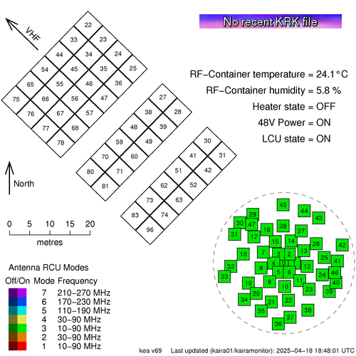
KAIRA Status Map

We have a new status map showing the situation with KAIRA.

This shows the actual current status:

This is available from the Status page, which can be found in the title bar of this web log.

The map shows the array layout of the antennas. The High-Band Antenna (HBA) tiles are in the top left and the Low-Band Antenna (LBA) aerials are in the lower right.   The layout is to scale, which is shown, and the direction to the VHF transmitter at Tromsø, is also indicated.

The antennas are numbered and they are also colour coded to show the Receiver Unit (RCU) mode. KAIRA has 96 RCUs and the RCU mode indicates which combination of antenna plus band-pass filter is used for the processing. Sometimes the entire array is configured to a single RCU mode and at other times it is mixed with several different modes for different antennas.

If an antenna is enabled, then the colour is bright, but if it is switched off, then it is dulled down.

In the case of a plain grey antenna icon, this means the antenna is shut down, either for maintenance, or as a result of damage.

Sometimes an antenna might be shaded with two colours like a two-tone maritime-Z-pennant. This is because each antenna has two polarisations, and there will be occasions when the RCU number/status for each polarisation is not the same.

In the bottom left, there is the legend and in the top right is the status label and the current RF-container parameters.

The image at the start of this post is "live". If you update the page, you might see ti change, depending on what KAIRA is doing. But to give an indication of what the status map might look like, here are some other static examples:

A "357"-mode solar observation. The grey antennas
are those knocked out by the March 2014 blizzard.

A mode-3 riometry observation. Storm-damaged antennas
are also present in this particular example.

Saving and loading data in Python with JSON

Scroll down if you just want to see the example code.

Long-winded pre-amble about computer documentation

If you don't use a computer language too often, then they can be pretty baffling when you come back to them after time away coding up something else. Furthermore, you might find yourself stuck in the mindset (and terminology) of the other language, which makes it pretty difficult to search for the correct terms on the Internet.

Recently, I had just this problem. It was a simple problem.

In Python, I have a record structure (= dictionary) which has labels (= keys) and data (= values). I just want to save it to disk and then later read it back again. That's not so bad, but the one extra point is that I'd like the save file to human-readable, so I can quickly check it with an editor to either see what's there or make corrections.

I quickly decided that "json" was what I needed, instead of  "pickle" (not human-readable files) or csv (seemed to require more work to write out the file). Whether that was the right choice or not is neither here nor there. The fact is that I couldn't quite get it to work.

You see, the json documenation (LINK) while comprehensive doesn't match the terminology I was thinking in my head. Look for the phrase "save to disk" on that page and there is nothing. The word "save" simply does not appear.

Also, if you are used to simple terms like load, save, read, write, etc., then that documentation doesn't read so well. Seriously... go to that page, start at the heading and read it out loud and either listen to yourself and let someone else listen to it. Read to at least the end of the first example.

See what I mean?

Checking websites like StackOverflow finds others occasionally asking similar questions, but with aggressive/arrogant answers along the lines of "the documentation is fine, what's your problem? RTM!"

Well, sometimes we are just on the way to something else. We are scripting, not coding. And we need something in a hurry. We simply don't have the time/skill/experience to get our heads around nested associative array object stream hierarchies (or whatever).

Don't get me wrong. The Python documentation is very good. It is thorough and comprehensive. But if you are coming to it raw and with a problem already in mind, then it can be a bit impenetrable at times. And I have been programming for years and have written many hundreds of thousands of lines of code in various other languages, so I'd hate to think what it would be like for a complete novice.

In any case, if some search engine just happens to put up this weblog post and help one other person in the world who wants a quick and easy, fully working, example of how to write some data to disk and read it back in again, then I'll be happy!   :-)

Saving a Python dictionary to disk using JSON

Okay, here's the code I came up with...

#!/usr/bin/python

# This only uses the json package
import json

# Create a dictionary (a key-value-pair structure in Python)
my_dict = {                   
  'Name':      'KAIRA',
  'Location':  u'Kilpisj\u00E4rvi',
  'Longitude': 20.76,
  'Latitude':  69.07
}

# We can print the dictionary to show we have data. E.g.
print my_dict                 
print my_dict['Location']     

# Open a file for writing
out_file = open("test.json","w")

# Save the dictionary into this file
# (the 'indent=4' is optional, but makes it more readable)
json.dump(my_dict,out_file, indent=4)                                    

# Close the file
out_file.close()

At this point, my little programme has created a file called "test.json". The contents of it look like this...

{
    "Latitude": 69.07, 
    "Name": "KAIRA", 
    "Longitude": 20.76, 
    "Location": "Kilpisj\u00e4rvi"
}

You can edit this as a text file or print it to screen with Linux utilities like 'cat' or 'more'. It can be e-mailed too.

You can tweak the "indent" parameter to change the number of spaces, and there are other options in the json.dump() which can also be used to control the behaviour.

There are some complications if you have non-standard dictionaries or weird data types. You will probably also hit performance issues if you try to save vast quantities of data. However, for the purposes of something quick and simple, this was sufficient for me.

Loading a JSON file into a Python dictionary

Having saved our data, we need to read it back in again. I've done this as a separate programme.

#!/usr/bin/python

# This only uses the json package
import json

# Open the file for reading
in_file = open("test.json","r")

# Load the contents from the file, which creates a new dictionary
new_dict = json.load(in_file)

# Close the file... we don't need it anymore  
in_file.close()

# Print the contents of our freshly loaded dictionary
print new_dict

So, there you go. I hope that helps!

Observing tips #5 -- Checking Python versions

There is a lot of software that is used by LOFAR stations which is written in the Python computing language. While it is certainly a well-used and well-established software environment, there are certainly occasions when knowing the exact version of the libraries that you are using is very helpful.

In the case of KAIRA, we also use LOFAR software (and much of our software is conversely applicable to other LOFAR stations). So, there are occasions where we need to check on the version of a given installation.

To do this, we have this small Python programme which we use to check.

#!/usr/bin/python

import sys
import numpy
import scipy
import ephem
import matplotlib

print "Installed versions..."
print "python =",sys.version
print "numpy =",numpy.version.version
print "scipy =",scipy.version.version
print "(py)ephem =",ephem.__version__
print "matplotlib =",matplotlib.__version__

Simply run it, and it will print out the version numbers of the typically used packages: Python itself, NumPy, SciPy, PyEphem and MatPlotLib.

When I ran it just now on one of the KAIRA machines, I read the following:

~> ./swversion.py
Installed versions...
python = 2.7.3 (default, Apr 10 2013, 06:20:15)
[GCC 4.6.3]
numpy = 1.6.1
scipy = 0.9.0
(py)ephem = 3.7.5.1
matplotlib = 1.1.1rc
~> 

We hope that helps!

DistroAstro

Many astronomers use Linux. It is a powerful, portable and open operating system that is readily available (i.e. free and runs on most hardware). The KAIRA software (from the control system through to the data reduction) runs on a Linux system. However, Linux is also an interesting choice for general astronomy users.

Now, there is a Linux "distro" (= distribution) specifically tailored to the astronomy enthusiast. It is called "AstroDistro" and is available from http://www.distroastro.org/ . The latest release has just been made (v1.0.2, 09-Aug-2013) and details can be found on the web site.

Even if you don't install it, it is useful to whip through the slideshow presentation and see what sorts of interesting software can be run on Linux (not just AstroDistro, but many other distributions as well).

Astropy python library

In the past week, the main reference paper for the Astropy programming toolkit has been released. Quoting from that paper:

The Python programming language has become one of the fastest-growing programming languages in the astronomy community in the last decade. While there have been a number of efforts to develop Python packages for astronomy-specific functionality, these efforts have been fragmented, and several dozens of packages have been developed across the community with little or no coordination. This has led to duplication and a lack of homogeneity across packages, making it difficult for users to install all the required packages needed in an astronomer's toolkit. Because a number of these packages depend on individual or small groups of developers, packages are sometimes no longer maintained, or simply become unavailable, which is detrimental to long-term research and reproducibility.

Motivated by these issues, the Astropy project was started in 2011 out of a desire to bring together developers across the field of astronomy in order to coordinate the development of a common set of Python tools for astronomers and simplify the landscape of available packages. One of the primary aims of the Astropy project is to develop a core astropy package that covers much of the astronomy-specific functionality needed by researchers, complementing more general scienti c packages such as NumPy and SciPy, which are invaluable for numerical array-based calculations and more general scientific algorithms (e.g. interpolation, integration, clustering).

{Astropy}... covers units and unit conversions, absolute dates and times, celestial coordinates, tabular and gridded data, common astronomical file formats world coordinate system transformations, and cosmological utilities

More information can be found on the Astropy website: http://www.astropy.org/

Or from the reference paper itself: http://arxiv.org/abs/1307.6212

KAIRA beamlet statistics plotting programme

During the summer months, Sodankylä Geophysical Observatory runs a student/worker programme, which gives an opportunity to youngsters to gain valuable work experience (and earn a bit of money too). One of our summer workers this year, was Taavi Vierinen, who we asked to take on a task of writing some software to merge and plot KAIRA beamlet statistics (BST) files.

Taavi accomplished this task very well and produced an excellent result. He also learned a lot in the process, not just about KAIRA and our geophysics, but also about programming and software engineering techniques. (He also taught us a thing or two!).

Today was Taavi's last day at the observatory. Before departing, he wrote this small report, in addition to the rest of the software documentation, which we are including as today's KAIRA web log post.

Taavi writes about his software:

This program combines two BST files into a single one, the program can also be used to plot an image from a single file. Data taken from the two files is controlled by user input, giving the program time from last N seconds as variable. The program then detects the relevant files and takes copies the data, amount specified by the given time from the chronologically first file, if it doesn't have enough data, the program then continues to second file and copies the remainder from there. If there is no file from the day specified, the program will use file filled with 'scrap data' to create empty data in its place, the scrap data is one hour of information copied from a random BST file repeated 24 times to get 24 hours amount of data. If neither of the two files is found, the program will still plot an image, but it will be fully black graph representing that there is no data from given period.

Sample plots... click to enlarge. (Image: T. Vierinen)

After the temporary file is created, the code made by Derek kicks in and uses the data to create a graph. Only changes I made there were few lines of code that would draw a black box on the scrap data and one that draws a line to position where the data from different files meet, so it is easier to see from which day the data originally came.

In the screenshot there are images which were drawn by the program: reference (1), (2) and (3).

• In reference(1) you can see what is drawn when both of the relevant files are found, if data from only a single file is used, the image will be similar, but it won't have the white line as there is only a single file as its source.
• In reference(2) you can see what the image looks like when the latest file doesn't exist. The program draws black box in its place, for 24 hours worth of samples.
• In reference(3) the situation is reversed from reference(2), this time the oldest of the two wanted files doesn't exist, note that in both reference(2) and reference(3), the white line separating the data from different source can be seen.

The program was created using python 2.7.5, by both me, Taavi Vierinen, and Derek McKay-Bukowski. I enjoyed this project, because I managed to learn a lot of skills from it, from using python to managing what I did on my spare time. The project was good to me in many ways and it wasn't too easy either, nor too difficult!

-Taavi Vierinen

Thanks for all your efforts Taavi and well done on the project. Have a safe trip back down south and we wish you all the best.

To you, and all our readers, have a nice weekend!