 |
| KAIRA data systems (Photo: D. McKay-Bukowski) |

Showing posts with label data. Show all posts
Showing posts with label data. Show all posts
Monday, 25 August 2014
Data extraction
There are numerous computers in the RF-container, which handle data processing, control and storage. One of these has now been taken out and has been moved back to SGO for use there in some of our interferometric riometry development work. During the extraction of this data system, we had the side cover of the RF-container signal processing racks off, thus once can see the other computers, network gear, etc.

Sunday, 15 June 2014
KAIRA EISCAT VHF intersection heights/elevations
In order for the KAIRA beam to intersect the vertical EISCAT VHF transmitter beam, the elevation must be set as follows. (All data provided by I.I.Virtanen, U. Oulu).


Note that the azimuth to the EISCAT VHF is 313.95 degrees. The numbers for the above plots are as follows. Hgt is the height above the EISCAT VHF transmitter in kilometres and Elev is the require elevation of observation from KAIRA to have the beam centre at this height.
We hope you read all these numbers and memorised them!
Note that the azimuth to the EISCAT VHF is 313.95 degrees. The numbers for the above plots are as follows. Hgt is the height above the EISCAT VHF transmitter in kilometres and Elev is the require elevation of observation from KAIRA to have the beam centre at this height.
| Hgt | Elev | Hgt | Elev | Hgt | Elev |
| 0 | -0.735 | 670 | 82.155 | 1340 | 85.69 |
| 10 | 6.101 | 680 | 82.259 | 1350 | 85.717 |
| 20 | 12.747 | 690 | 82.359 | 1360 | 85.743 |
| 30 | 19.044 | 700 | 82.457 | 1370 | 85.768 |
| 40 | 24.881 | 710 | 82.552 | 1380 | 85.793 |
| 50 | 30.199 | 720 | 82.644 | 1390 | 85.818 |
| 60 | 34.987 | 730 | 82.734 | 1400 | 85.843 |
| 70 | 39.261 | 740 | 82.821 | 1410 | 85.867 |
| 80 | 43.06 | 750 | 82.906 | 1420 | 85.891 |
| 90 | 46.431 | 760 | 82.989 | 1430 | 85.914 |
| 100 | 49.423 | 770 | 83.07 | 1440 | 85.937 |
| 110 | 52.082 | 780 | 83.148 | 1450 | 85.96 |
| 120 | 54.451 | 790 | 83.225 | 1460 | 85.982 |
| 130 | 56.568 | 800 | 83.3 | 1470 | 86.005 |
| 140 | 58.467 | 810 | 83.373 | 1480 | 86.027 |
| 150 | 60.176 | 820 | 83.444 | 1490 | 86.048 |
| 160 | 61.719 | 830 | 83.513 | 1500 | 86.069 |
| 170 | 63.117 | 840 | 83.581 | 1510 | 86.09 |
| 180 | 64.39 | 850 | 83.648 | 1520 | 86.111 |
| 190 | 65.551 | 860 | 83.712 | 1530 | 86.132 |
| 200 | 66.613 | 870 | 83.776 | 1540 | 86.152 |
| 210 | 67.589 | 880 | 83.837 | 1550 | 86.172 |
| 220 | 68.488 | 890 | 83.898 | 1560 | 86.192 |
| 230 | 69.318 | 900 | 83.957 | 1570 | 86.211 |
| 240 | 70.087 | 910 | 84.015 | 1580 | 86.23 |
| 250 | 70.801 | 920 | 84.072 | 1590 | 86.249 |
| 260 | 71.465 | 930 | 84.127 | 1600 | 86.268 |
| 270 | 72.084 | 940 | 84.181 | 1610 | 86.287 |
| 280 | 72.663 | 950 | 84.234 | 1620 | 86.305 |
| 290 | 73.205 | 960 | 84.286 | 1630 | 86.323 |
| 300 | 73.714 | 970 | 84.337 | 1640 | 86.341 |
| 310 | 74.192 | 980 | 84.387 | 1650 | 86.358 |
| 320 | 74.642 | 990 | 84.436 | 1660 | 86.376 |
| 330 | 75.067 | 1000 | 84.484 | 1670 | 86.393 |
| 340 | 75.468 | 1010 | 84.531 | 1680 | 86.41 |
| 350 | 75.847 | 1020 | 84.577 | 1690 | 86.427 |
| 360 | 76.207 | 1030 | 84.622 | 1700 | 86.443 |
| 370 | 76.548 | 1040 | 84.667 | 1710 | 86.46 |
| 380 | 76.872 | 1050 | 84.71 | 1720 | 86.476 |
| 390 | 77.18 | 1060 | 84.753 | 1730 | 86.492 |
| 400 | 77.473 | 1070 | 84.795 | 1740 | 86.508 |
| 410 | 77.752 | 1080 | 84.836 | 1750 | 86.523 |
| 420 | 78.019 | 1090 | 84.876 | 1760 | 86.539 |
| 430 | 78.274 | 1100 | 84.916 | 1770 | 86.554 |
| 440 | 78.518 | 1110 | 84.955 | 1780 | 86.569 |
| 450 | 78.751 | 1120 | 84.993 | 1790 | 86.584 |
| 460 | 78.974 | 1130 | 85.031 | 1800 | 86.599 |
| 470 | 79.188 | 1140 | 85.067 | 1810 | 86.614 |
| 480 | 79.394 | 1150 | 85.104 | 1820 | 86.628 |
| 490 | 79.591 | 1160 | 85.139 | 1830 | 86.643 |
| 500 | 79.781 | 1170 | 85.174 | 1840 | 86.657 |
| 510 | 79.963 | 1180 | 85.209 | 1850 | 86.671 |
| 520 | 80.139 | 1190 | 85.243 | 1860 | 86.685 |
| 530 | 80.308 | 1200 | 85.276 | 1870 | 86.698 |
| 540 | 80.471 | 1210 | 85.309 | 1880 | 86.712 |
| 550 | 80.628 | 1220 | 85.341 | 1890 | 86.725 |
| 560 | 80.78 | 1230 | 85.373 | 1900 | 86.739 |
| 570 | 80.927 | 1240 | 85.404 | 1910 | 86.752 |
| 580 | 81.068 | 1250 | 85.435 | 1920 | 86.765 |
| 590 | 81.205 | 1260 | 85.465 | 1930 | 86.778 |
| 600 | 81.337 | 1270 | 85.495 | 1940 | 86.79 |
| 610 | 81.466 | 1280 | 85.524 | 1950 | 86.803 |
| 620 | 81.59 | 1290 | 85.553 | 1960 | 86.815 |
| 630 | 81.71 | 1300 | 85.581 | 1970 | 86.828 |
| 640 | 81.826 | 1310 | 85.609 | 1980 | 86.84 |
| 650 | 81.939 | 1320 | 85.636 | 1990 | 86.852 |
| 660 | 82.049 | 1330 | 85.664 | 2000 | 86.864 |
We hope you read all these numbers and memorised them!
Wednesday, 11 June 2014
Double-X-flare
Yesterday morning we were meant to do incoherent scatter radar (ISR) observations of the EISCAT VHF. This was in conjunction with a demonstration/prototype system that is also being tested at the KAIRA site (more on this in a forthcoming article!). Then, in the afternoon, we'd revert to solar observing.
However, due to various issues we ended up postponing the VHF ISR observations to the afternoon. Sure enough during that time there was two X-class solar flares. Yep, not one, but two. After months of radio silence what there the chances (pretty good, it seems!).

In any case we were observing nonetheless and there was a chance we might have seen something in the sidelobes of the tile beams. Sure enough there were several hints of natural emission, which may be from the sun.


However, due to various issues we ended up postponing the VHF ISR observations to the afternoon. Sure enough during that time there was two X-class solar flares. Yep, not one, but two. After months of radio silence what there the chances (pretty good, it seems!).
In any case we were observing nonetheless and there was a chance we might have seen something in the sidelobes of the tile beams. Sure enough there were several hints of natural emission, which may be from the sun.
Monday, 19 May 2014
Further investigations on the strange solar ripple
We've been following the progress on trying to understand a strange ripple in some recent solar observations.
As each antenna has two polarisations, we plot first the X-polarisation and the Y-polarisation. They are done separately, to avoid a strong flickering effect (which is due to the different responses to the event between the two polarisations).
The "RCU" number is the Reciever Unit number. The even RCUs are for the X-polarisation and the odd ones are for the Y-polarisation. Three RCUs have been omitted (68,69, and 70) as these were offline at the time the observations were made.
Actually, we noticed that they oscillate. The oscillation is small to start with and then it increases. The movement is small, but those fringes waver with RCU number.
RCU number is a function of the antenna number.
RCU 0,1 = LBA #L00
RCU 2,3 = LBA #L01
:
:
RCU 94,95 = LBA #L47
And, if you look at the map of the array, and join the dots in numeric order, you get this:

So, then what I did was to look for where the minimum fringes and maximum fringes occur. In other words, as the pattern moves up and down, what are the local min/max points in that oscillation.
I noted the RCU numbers, determined the antenna numbers and plotted them. I also note the direction of the sun during this time (roughly).

This tells as that the fringe pattern is associated with distance from the sun. Well, it is not likely to be that directly, but because there is a mound with the LBAs, there will be more flat ground between #L43 and the sun than #L35. This snow/ground could be causing reflections.
What these results tell us, though, is that the original hypothesis of a reflection off the reindeer fence or gate is actually pretty unlikely.
So there are now two likes of thought. One is that this is a snow effect and some modelling is going on to investigate this.
The other is that it is an ionospheric refraction effect.
Neither idea is firm yet and investigations remain ongoing.
As each antenna has two polarisations, we plot first the X-polarisation and the Y-polarisation. They are done separately, to avoid a strong flickering effect (which is due to the different responses to the event between the two polarisations).
The "RCU" number is the Reciever Unit number. The even RCUs are for the X-polarisation and the odd ones are for the Y-polarisation. Three RCUs have been omitted (68,69, and 70) as these were offline at the time the observations were made.
Actually, we noticed that they oscillate. The oscillation is small to start with and then it increases. The movement is small, but those fringes waver with RCU number.
RCU number is a function of the antenna number.
RCU 0,1 = LBA #L00
RCU 2,3 = LBA #L01
:
:
RCU 94,95 = LBA #L47
And, if you look at the map of the array, and join the dots in numeric order, you get this:
So, then what I did was to look for where the minimum fringes and maximum fringes occur. In other words, as the pattern moves up and down, what are the local min/max points in that oscillation.
I noted the RCU numbers, determined the antenna numbers and plotted them. I also note the direction of the sun during this time (roughly).
This tells as that the fringe pattern is associated with distance from the sun. Well, it is not likely to be that directly, but because there is a mound with the LBAs, there will be more flat ground between #L43 and the sun than #L35. This snow/ground could be causing reflections.
What these results tell us, though, is that the original hypothesis of a reflection off the reindeer fence or gate is actually pretty unlikely.
So there are now two likes of thought. One is that this is a snow effect and some modelling is going on to investigate this.
The other is that it is an ionospheric refraction effect.
Neither idea is firm yet and investigations remain ongoing.
Monday, 5 May 2014
Curious ripple in the data
The strange ripple in the dynamic spectrum of the solar radio event from a few weeks back has caught some interest, and we don't have an explanation for it... yet. At first, it was thought it might be an RFI effect, although it is very broad. It also drifts in frequency, which is unusual.
These data are from a single dipole. So, it might be coupling between that and other dipoles, or perhaps Cas A rippling through a sidelobe. For the UK station (which doesn't see the effect -- REF), these sources would be at different position angles. There are several things we have now checked:
We see it on different dipoles. These might have different couplings (due to antenna spacings) or be at different position angles (with respect to, say, a local RFI source).
We also see it on both polarisations. The following two plots are from different polarisations.
We may still be seeing some sort of ground effect or perhaps a reflection from the reindeer fence. Alternatively, it might be a "snow interferometer" (like the old sea-interferometer, but with a reflection off the snow). The fact is that the sun is at quite a low elevation and the wavelengths are quite long at these frequency bands.
In any case, we remain puzzled. Any suggestions, anyone?
These data are from a single dipole. So, it might be coupling between that and other dipoles, or perhaps Cas A rippling through a sidelobe. For the UK station (which doesn't see the effect -- REF), these sources would be at different position angles. There are several things we have now checked:
We see it on different dipoles. These might have different couplings (due to antenna spacings) or be at different position angles (with respect to, say, a local RFI source).
We also see it on both polarisations. The following two plots are from different polarisations.
 |
| LBA aerial #L04, X-polarisation (Image: D. McKay-Bukowski) |
 |
| LBA aerial #L04, Y-polarisation (Image: D. McKay-Bukowski) |
We may still be seeing some sort of ground effect or perhaps a reflection from the reindeer fence. Alternatively, it might be a "snow interferometer" (like the old sea-interferometer, but with a reflection off the snow). The fact is that the sun is at quite a low elevation and the wavelengths are quite long at these frequency bands.
In any case, we remain puzzled. Any suggestions, anyone?
Saturday, 3 May 2014
Using median filters in quicklook plots
When we make our plots of spectrum vs. time, we often use a median filter to improve the contrast. The reason for the median filter is that the amplifiers have a certain
spectral response associated with them. What you are interested in is the
proportional variation of the signal with respect to what it would be if
there was no signal.
You can do this by really careful bandpass calibration, but for "quicklook" plots, dividing by the median works and it is very quick. So that's what I use for these plots that I put on the web.
The Python code fragment looks like this:
Here, "data" is a 2D array with the axes being subband and time.
If you didn't use a median filter, you would expect to see a strong band at about subband 300 (approx. 55-60 MHz). This is due to the peak response of the amplifiers at that region (EXAMPLE). By using the median filter, you remove this bias.
Of course, you still need to be careful. The median filter relies on their being a stable background and more background than signal. In the first plot above, there is a slight negative band around 55-60 MHz, as there was probably a bit too much signal, thus skewing the data. For the purposes of seeing the features, it is not too much of a problem though.
The only way to really do this is with a full bandpass calibration but, as mentioned, for a quicklook the median filter gives you a good, easy, high-contrast plot.
You can do this by really careful bandpass calibration, but for "quicklook" plots, dividing by the median works and it is very quick. So that's what I use for these plots that I put on the web.
 |
| Some subband statistics with a median filter. |
 |
| The same data, but without the filter. |
The Python code fragment looks like this:
        # Determine the median
        med=np.median(data, axis=1)

        # Apply the median to the data
        for i in xrange(data.shape[1]): data[:,i] /= med
Here, "data" is a 2D array with the axes being subband and time.
If you didn't use a median filter, you would expect to see a strong band at about subband 300 (approx. 55-60 MHz). This is due to the peak response of the amplifiers at that region (EXAMPLE). By using the median filter, you remove this bias.
Of course, you still need to be careful. The median filter relies on their being a stable background and more background than signal. In the first plot above, there is a slight negative band around 55-60 MHz, as there was probably a bit too much signal, thus skewing the data. For the purposes of seeing the features, it is not too much of a problem though.
The only way to really do this is with a full bandpass calibration but, as mentioned, for a quicklook the median filter gives you a good, easy, high-contrast plot.
Monday, 21 April 2014
Spectacular solar radio event
Last Friday, KAIRA observed the most amazing radio event from the sun. There was a strong X-ray event, which corresponded to an amazing multi-frequency solar event in the radio. The following plot is from the GOES X-ray monitor (source: NOAA/SWPC)

The event was detected at KAIRA and the following plot shows the entire event sequence.
The initial event was preceded by a smaller, fainter event. However the first of the strong radio bursts was very strong and mostly uniform in frequency distribution.
The subsequent events were much more complicated. In particular, there was a very slowly decaying radio event, which cascaded down through the different frequencies of the Low-Band Array (which was operating at the time).
What is really curious is the ripple effect through the different frequencies. Is this an interferometric effect from the coupling between antennas? However, these data were taken with a single LBA aerial.
It will be interesting to see what auroral activity occurs over the next few days. Although it is getting close to the midnight-sun season, KAIRA will be able to monitor the events using the new riometry modes.
Overall it was a very interesting event. We will be conducting a number of dedicated solar observing events over the summer with KAIRA, so hope to report on more solar data in the next few months.
The event was detected at KAIRA and the following plot shows the entire event sequence.
 |
| KAIRA detecting of the solar radio event (Image: D. McKay-Bukowski) |
The initial event was preceded by a smaller, fainter event. However the first of the strong radio bursts was very strong and mostly uniform in frequency distribution.
 |
| Zooming in on the initial event (Image: D. McKay-Bukowski) |
The subsequent events were much more complicated. In particular, there was a very slowly decaying radio event, which cascaded down through the different frequencies of the Low-Band Array (which was operating at the time).
 |
| The main event... very complex! (Image: D. McKay-Bukowski) |
What is really curious is the ripple effect through the different frequencies. Is this an interferometric effect from the coupling between antennas? However, these data were taken with a single LBA aerial.
It will be interesting to see what auroral activity occurs over the next few days. Although it is getting close to the midnight-sun season, KAIRA will be able to monitor the events using the new riometry modes.
Overall it was a very interesting event. We will be conducting a number of dedicated solar observing events over the summer with KAIRA, so hope to report on more solar data in the next few months.
Wednesday, 12 February 2014
Snow on the LBA field
Over the last couple of days, we've reported how snow affects the RF performance of the LBA aerials. Today we have some more photographs from #L33 and #L34.
 |
| Just a bit deeper here. Note how this aerial has its wires partly covered, where the others in the background have their guys and elastics still visible above the snow line. (Photo: D. McKay-Bukowski) |
 |
| There was about 20 cm of ice along each receiver wire. (Photo: D. McKay-Bukowski) |
 |
| Another image of the iced up wire. The snow depth is approx. 70-75 cm. The HBA array is visible in the background. (Photo: D. McKay-Bukowski) |
 |
| Digging down to the ground plane. Notice how the aerial is leaning. This is due to the ice tension on the wires, guys and elastics, causing distortion of the LBA aerial. |
Tuesday, 11 February 2014
Snow affecting the RF-performance
Yesterday we showed a plot which indicated strange spectral responses of the LBA aerials #L33 and #L34. Today we show what is causing this strange effect...
Snow.
Each LBA aerial has four wires that descend from the top of the aerial down towards the corner pegs. This is the receiving wires. However, the lower part is just for support and is either nylon or elastic. As long as the snow is below that level, it does not affect the performance of the wires to receive the radio waves.
The wires reach down to approx. 65 cm above the ground. But, if the snow depth exceeds 65 cm, then this partial covering will start to affect the antenna. And this is precisely what happened to aerials #L33 and #L34.
Snow.
Each LBA aerial has four wires that descend from the top of the aerial down towards the corner pegs. This is the receiving wires. However, the lower part is just for support and is either nylon or elastic. As long as the snow is below that level, it does not affect the performance of the wires to receive the radio waves.
The wires reach down to approx. 65 cm above the ground. But, if the snow depth exceeds 65 cm, then this partial covering will start to affect the antenna. And this is precisely what happened to aerials #L33 and #L34.
 |
| The author inspecting #L34. The snow depth here is 70 cm. |
Monday, 10 February 2014
Strange subband responses
Data Monday again. This time we're featuring some subband statistics from KAIRA's Low-Band Antenna (LBA) array.
There are 48 aerials and for each of these there are two polarisations. Thus, there are 96 signals coming back from the array. Each one has its own Receiver Unit (RCU). After filtering, the signals are digitised and split into 512 frequency channels, called subbands. 1-second average power for each subband for each RCU is calculated and recorded. These are the subband statistics and they can be used for form a spectrum for each RCU, to show its performance. We've occasionally shown these before.
However, last week we noticed something a bit odd...
Four of the RCUs were showing low signals. These were numbers 65, 66, 67 and 68. Here's a plot showing them. Also shown in the plot are RCUs 64 and 65 (which are behaving correctly).
The forest of vertical lines towards the left is radio-frequency interference (RFI) from shortwave radio. The two near the right are FM radio stations. We do expect a peak towards 55-60 MHz, which is the best response for the amplifiers and antenna design. However, notice how RCUs 67, 68 and 69 have their peak shifted to the left a bit. And RCU 66 has a double peak.
Very strange.
If we look up the LBA aerial numbers associated with these RCUs, we find that RCUs 66,67 are for LBA #L33. And 68,69 are for LBA #L34. And, if we check the array map, we find that these two aerials are on the southwestern edge of the LBA array.
Well, we've now done some investigations and have found the cause of the problem. But we'll save that for tomorrow. Until then, you can speculate for yourself. :-)
There are 48 aerials and for each of these there are two polarisations. Thus, there are 96 signals coming back from the array. Each one has its own Receiver Unit (RCU). After filtering, the signals are digitised and split into 512 frequency channels, called subbands. 1-second average power for each subband for each RCU is calculated and recorded. These are the subband statistics and they can be used for form a spectrum for each RCU, to show its performance. We've occasionally shown these before.
However, last week we noticed something a bit odd...
Four of the RCUs were showing low signals. These were numbers 65, 66, 67 and 68. Here's a plot showing them. Also shown in the plot are RCUs 64 and 65 (which are behaving correctly).
 |
| KAIRA subband statistics 05-Feb-2014. RCUs 64 & 65 are behaving normally. The others are a bit odd. |
The forest of vertical lines towards the left is radio-frequency interference (RFI) from shortwave radio. The two near the right are FM radio stations. We do expect a peak towards 55-60 MHz, which is the best response for the amplifiers and antenna design. However, notice how RCUs 67, 68 and 69 have their peak shifted to the left a bit. And RCU 66 has a double peak.
Very strange.
If we look up the LBA aerial numbers associated with these RCUs, we find that RCUs 66,67 are for LBA #L33. And 68,69 are for LBA #L34. And, if we check the array map, we find that these two aerials are on the southwestern edge of the LBA array.
Well, we've now done some investigations and have found the cause of the problem. But we'll save that for tomorrow. Until then, you can speculate for yourself. :-)
Monday, 2 December 2013
SFIR coverage
Hmm... data Monday again. Where did that weekend just go?
We had some visitors from Linz, Austria visit the KAIRA site on Friday. It was great to show them around as they asked lots of interesting questions (and I had a great chance to practice my now-very-rusty Deutsch). Most of the questions were about the imaging, which I've shown countless times on this weblog.
However, there was one screen which went uncommented...
This screen uses old-fashioned ASCII-art to show the coverage of one of our imaging riometry projects (SFIR). The lines refer to the day of the observation (e.g. 20130920 = 20-Jul-2013) and the columns are the hours of the day.
Then, for each position, there is a number from 0 to 9, or a blank or a hash (#). The blanks are where no data has yet been processed. The has shows the hours for which complete processing has occurred. The others show a fraction where 0 = 0-9%, 1 = 10-19%, 2 = 20-29% up to 9 = 90-99%.
As the processing continues, this chart will slowly fill up. However, with huge transforms, massive data sets and a lot of time, this will still take some four to five weeks of processing time on one of the powerful KAIRA computers.
However, it is nice to still see old-fashioned ASCII displays. Reminds me of the old days...
We had some visitors from Linz, Austria visit the KAIRA site on Friday. It was great to show them around as they asked lots of interesting questions (and I had a great chance to practice my now-very-rusty Deutsch). Most of the questions were about the imaging, which I've shown countless times on this weblog.
However, there was one screen which went uncommented...
 |
| Imaging coverage (Image: D. McKay-Bukowski) |
Then, for each position, there is a number from 0 to 9, or a blank or a hash (#). The blanks are where no data has yet been processed. The has shows the hours for which complete processing has occurred. The others show a fraction where 0 = 0-9%, 1 = 10-19%, 2 = 20-29% up to 9 = 90-99%.
As the processing continues, this chart will slowly fill up. However, with huge transforms, massive data sets and a lot of time, this will still take some four to five weeks of processing time on one of the powerful KAIRA computers.
However, it is nice to still see old-fashioned ASCII displays. Reminds me of the old days...
Monday, 14 October 2013
KAIRA data rates
KAIRA is capable of producing different types of data files, depending on the configuration of the software and hardware control parameters. These different data types are suited to different experiments and it is not necessary (or even desirable) to record all of them.
There are standard data products, which are the statistics files generated by the standard LOFAR system. These are typically used for programmes such as riometry, solar observing, scintillation experiments, station calibration, and so on. These standard data products are as follows:
SST -- Subband-Statistics
These record a 1-second average power, for each subband, for each of the 96 receiver units (RCU). This produces 96 files, with N records (where N is the number of seconds), where each record is 512 subbands in size.
BST -- Beamlet Statistics
These are 1-second average power, for each beamlet for each polarisation. There are either 244x16-bit, 488x8-bit or 976x4-bit beamlets. (In reality the 16-bit beamlets only have 12-bits of dynamic range, but are still packed into 16-bit words). This produces two files (X and Y polarisation), with N records (where N is the number of seconds), where each record is B beamlets in size.
ACC -- Array Covariance Cubes
ACC files (also sometimes referred to as Antenna Cross-Correlation) files contain visibility data for all the baseline pairs within the array, averaged to 1 second.
XST -- Cross-correlation Statistics
Similar to ACC files, but these record each second a single subband, rather than stepping through them. Additionally, rather than resetting and starting a new file after 512 seconds, it records continuously. Note that it is not possible to recrod both ACC and XST files at the same time.
Data rates
It is important that observers appreciate how much data KAIRA can record, so that data storage and transport can be appropriately managed. The following table summarises the rates, assuming a standard configuration:
In addition to the standard data products, KAIRA can also record raw voltage level data. These are typically recorded with programmes such as KLP or KUG (but not both!). For these, the data rates can be extremely high and, as such, it does not make sense to indicate a daily total (as that would easily our existing on-site storage).
Please note that any experiment requiring raw voltage-level data will require these non-standard products. This includes Incoherent Scatter Radar (ISR) experiments and Very-Long Baseline Interferometry (VLBI) observations. In all such cases, data storage and handling will need to be coordinated with the KAIRA team. In large data-volume cases, observers will be expected to provide their own storage.
These represent maximum values. Sometimes we decimate the data (pulsar observing) or average it (interplanetary scintillation observations). These data can be taken in addition to standard data products.
References
Standard data products
There are standard data products, which are the statistics files generated by the standard LOFAR system. These are typically used for programmes such as riometry, solar observing, scintillation experiments, station calibration, and so on. These standard data products are as follows:
SST -- Subband-Statistics
These record a 1-second average power, for each subband, for each of the 96 receiver units (RCU). This produces 96 files, with N records (where N is the number of seconds), where each record is 512 subbands in size.
BST -- Beamlet Statistics
These are 1-second average power, for each beamlet for each polarisation. There are either 244x16-bit, 488x8-bit or 976x4-bit beamlets. (In reality the 16-bit beamlets only have 12-bits of dynamic range, but are still packed into 16-bit words). This produces two files (X and Y polarisation), with N records (where N is the number of seconds), where each record is B beamlets in size.
ACC -- Array Covariance Cubes
ACC files (also sometimes referred to as Antenna Cross-Correlation) files contain visibility data for all the baseline pairs within the array, averaged to 1 second.
XST -- Cross-correlation Statistics
Similar to ACC files, but these record each second a single subband, rather than stepping through them. Additionally, rather than resetting and starting a new file after 512 seconds, it records continuously. Note that it is not possible to recrod both ACC and XST files at the same time.
Data rates
It is important that observers appreciate how much data KAIRA can record, so that data storage and transport can be appropriately managed. The following table summarises the rates, assuming a standard configuration:
| Type | Files per day | Size per file | Daily total | Rate |
| SST | 96 | 352149504 | 33.8 GB | 391 kB/s |
| ACC | 164 | 75497472 | 12.4 GB | 143 kB/s |
| BST | 4 | 167821248 | 0.7 GB | 7.7 kB/s |
Non-standard data products
In addition to the standard data products, KAIRA can also record raw voltage level data. These are typically recorded with programmes such as KLP or KUG (but not both!). For these, the data rates can be extremely high and, as such, it does not make sense to indicate a daily total (as that would easily our existing on-site storage).
| Type | Files | Individual rate | Total rate |
| KUG | 4 | 96 MB/s | 383 MB/s |
| KLP | approx. 244/s | 90 MB/s | 380 MB/s |
Please note that any experiment requiring raw voltage-level data will require these non-standard products. This includes Incoherent Scatter Radar (ISR) experiments and Very-Long Baseline Interferometry (VLBI) observations. In all such cases, data storage and handling will need to be coordinated with the KAIRA team. In large data-volume cases, observers will be expected to provide their own storage.
These represent maximum values. Sometimes we decimate the data (pulsar observing) or average it (interplanetary scintillation observations). These data can be taken in addition to standard data products.
References
- "Computing for data acquisition", KAIRA document KAIRA-SGO-PRP-002.
- "LOFAR station data cookbook", ASTRON document LOFAR-ASTRON-MAN-064.
Thursday, 3 October 2013
Observing tips #5 -- Checking Python versions
There is a lot of software that is used by LOFAR stations which is written in the Python computing language. While it is certainly a well-used and well-established software environment, there are certainly occasions when knowing the exact version of the libraries that you are using is very helpful.
In the case of KAIRA, we also use LOFAR software (and much of our software is conversely applicable to other LOFAR stations). So, there are occasions where we need to check on the version of a given installation.
To do this, we have this small Python programme which we use to check.
Simply run it, and it will print out the version numbers of the typically used packages: Python itself, NumPy, SciPy, PyEphem and MatPlotLib.
When I ran it just now on one of the KAIRA machines, I read the following:
We hope that helps!
In the case of KAIRA, we also use LOFAR software (and much of our software is conversely applicable to other LOFAR stations). So, there are occasions where we need to check on the version of a given installation.
To do this, we have this small Python programme which we use to check.
#!/usr/bin/python

import sys
import numpy
import scipy
import ephem
import matplotlib
print "Installed versions..." print "python =",sys.version print "numpy =",numpy.version.version print "scipy =",scipy.version.version print "(py)ephem =",ephem.__version__ print "matplotlib =",matplotlib.__version__
Simply run it, and it will print out the version numbers of the typically used packages: Python itself, NumPy, SciPy, PyEphem and MatPlotLib.
When I ran it just now on one of the KAIRA machines, I read the following:
~> ./swversion.py
Installed versions...
python = 2.7.3 (default, Apr 10 2013, 06:20:15)
[GCC 4.6.3]
numpy = 1.6.1
scipy = 0.9.0
(py)ephem = 3.7.5.1
matplotlib = 1.1.1rc
~>
We hope that helps!
Monday, 23 September 2013
KAIRA operational status label
Over the last few months, we've had some occasional technical problems with KAIRA. That's all fixed now and the station is back online and observing again. However, the outages did highlight the fact that we could use some improved monitoring and also that this monitoring needs to be more visible.
So, as a result of this we've put a new monitoring tool in place which generates a display icon. This will be used in various places on our system for the benefit of staff, but we've also decided to put it on the web log too. Apart from being useful to our observers and the support staff, it may also be of interest to the general public and anyone else who might be interested in KAIRA's operational status.
When working well, the status icon will be pretty bland, with just some text indicating that it is operational and what the time of the last check was. It will look something like this:

Checks are made once a minute, so you should see it change if you were to reload the web page.
However, if something is not quite right, the background will change to a pretty eye-catching colour and the text will indicate the likely cause of the fault (or at least a pointer for the support team as to where they could start looking to work out what is wrong). Some examples include:


In summary, the status label will help improve uptime and let us catch and fix problems quickly. But it will also be a useful widget for users of the system too.
So, as a result of this we've put a new monitoring tool in place which generates a display icon. This will be used in various places on our system for the benefit of staff, but we've also decided to put it on the web log too. Apart from being useful to our observers and the support staff, it may also be of interest to the general public and anyone else who might be interested in KAIRA's operational status.
When working well, the status icon will be pretty bland, with just some text indicating that it is operational and what the time of the last check was. It will look something like this:
Checks are made once a minute, so you should see it change if you were to reload the web page.
However, if something is not quite right, the background will change to a pretty eye-catching colour and the text will indicate the likely cause of the fault (or at least a pointer for the support team as to where they could start looking to work out what is wrong). Some examples include:
In summary, the status label will help improve uptime and let us catch and fix problems quickly. But it will also be a useful widget for users of the system too.
Monday, 16 September 2013
KAIRA plasma parameter fit
Ilkka Virtanen and Niklas Siipola have been analysing some of the KAIRA data that was recorded during the previous Finnish EISCAT campaign. The following plots show bi-static incoherent scatter plasma parameter profile plots obtained using KAIRA. The results are in good agreement with the Tromsø measurements, and also show for the first time that a simultaneous bi-static plasma parameter profile can be obtained using a phased array incoherent scatter radar receiver. This is still work in progress, but this is yet another step in the direction of KAIRA performing routine incoherent scatter plasma parameter measurements.
The PI of the experiment was Anita Aikio and the purpose of the experiment was to 1) obtain the first tri-static EISCAT VHF measurements, and 2) to leverage the multi beam capability of KAIRA to obtain a profile of wind velocity vectors (due to the lack of a third station, only two components of the velocity vector can be obtained).
 |
| Plasma parameters obtained using KAIRA. |
 |
| Plasma parameters obtained using EISCAT VHF. |
Monday, 19 August 2013
Sunshine in the data
'Tis "Data Monday" again. Today, we've an example of where the radio-bright sun is showing up in one of the all-sky images.

Click on the plot to enlarge it.Note that this is an orthographic projection. Also, this is a "sky-view"... in other words, it is as if you are lying on your back in the middle of the array looking up. A few markers indicate some bright sources (Cas A and Cyg A) and directions (such as the direction to the VHF transmitter in Tromsø).
However, the one to look for is the very bright object at the bottom of the plot: radio emission from the sun.

Click on the plot to enlarge it.Note that this is an orthographic projection. Also, this is a "sky-view"... in other words, it is as if you are lying on your back in the middle of the array looking up. A few markers indicate some bright sources (Cas A and Cyg A) and directions (such as the direction to the VHF transmitter in Tromsø).
However, the one to look for is the very bright object at the bottom of the plot: radio emission from the sun.
Monday, 12 August 2013
Answer to the strange RFI
Data Monday again... so what was the answer to the strange RFI we reported a couple of weeks ago? Well, the best suggested we've had, is that it is Digital Audio Broadcast (DAB) radio from Norway. As each Each DAB multiplex has a bandwidth of about 1.536 MHz, that matches what we see in the data quite nicely. The propagation is probably via anomalous behaviour in the ionosphere (such as sporadic-E-layer).

The Tromsø transmitter is at 225.6 MHz and the Norwegian national transmitter is 229.07 MHz.
Reference: http://www.worlddab.org/country_information_/norway/multiplexes
Thanks to Juha Vierinen for finding these!

The Tromsø transmitter is at 225.6 MHz and the Norwegian national transmitter is 229.07 MHz.
Regional
Region: Nordland og Troms, Nordland og Troms
Transmitted on: Band III - 12B - 225.648MHz - (Nordland og Troms)
National
Norge Riks
Transmitted on: Band III - 12D - 229.072MHz
Reference: http://www.worlddab.org/country_information_/norway/multiplexes
Thanks to Juha Vierinen for finding these!
Thursday, 8 August 2013
The repair in the data
Over the last few days, we've been reporting on the damage and repair work to KAIRA LBA aerial L17. This story started with the data and so that's how we'll end it. The image for today is the data trace from the day of the repair. Yes, the data acquisition was running throughout this time, so it is possible to see (in the radio spectrum) the repair taking place.

If you look carefully, you can see distortions in the data in data after the point when the aerial was re-erected. This was due me being right next to the aerial during that time as I attached the nylon line and O-ring and then did up the knots and attach the cable ties. In total the whole process took about 5 minutes... excluding the time before re-righting the aerial, as I prepared the various items.
What this does show, though, is that people walking around the aerials do make a difference! Thus wandering on to the field during observations is not without consequence.
However, more significantly for us is that the discovery and repair were made on the 1st August... over a month since the aerial fell. Of course one aerial in 48 is not going to be a dramatic effect in the beamformed data, which is what we normally look at, but still it is a concern that we didn't notice this earlier.
While there are some procedures that exist for the main LOFAR network to test data integrity, they are not really suitable for the operations at KAIRA. However, we are now devising some new software to allow us to easily and automatically monitor the individual RCU data and thus hopefully detect such problems if they occur in the future.

If you look carefully, you can see distortions in the data in data after the point when the aerial was re-erected. This was due me being right next to the aerial during that time as I attached the nylon line and O-ring and then did up the knots and attach the cable ties. In total the whole process took about 5 minutes... excluding the time before re-righting the aerial, as I prepared the various items.
What this does show, though, is that people walking around the aerials do make a difference! Thus wandering on to the field during observations is not without consequence.
However, more significantly for us is that the discovery and repair were made on the 1st August... over a month since the aerial fell. Of course one aerial in 48 is not going to be a dramatic effect in the beamformed data, which is what we normally look at, but still it is a concern that we didn't notice this earlier.
While there are some procedures that exist for the main LOFAR network to test data integrity, they are not really suitable for the operations at KAIRA. However, we are now devising some new software to allow us to easily and automatically monitor the individual RCU data and thus hopefully detect such problems if they occur in the future.
Tuesday, 6 August 2013
Fallen LBA aerial
Yesterday, we showed some subband statistics data that indicated that something had gone awry with RCU 034 and 035. Of course a LOFAR expert would recognise that these are adjacent RCUs, and thus pertain to the same antenna. Knowing the KAIRA system (or making an educated guess) you could tell that this was antenna 17. Furthermore the peak at around 60 MHz (and the fact that the frequency range was 0–100 MHz) meant that this was an LBA unit.
The next hint, was that RCU 035 took 3 seconds to fail but RCU 034 took only 1 second, starting a second after the first. This indicates a failure on the Y-polarisation first, and implies that this first failure on Y, led to the failure on X. Sure enough, that was indeed the cause.
Here is what we found on arrival at the site.
As the data suggests, one of the guys broke causing the aerial to fall. The first second would have the northwest line (the Y-polarisation with elastic) drop down. At this instance the X-polarisation is still intact. Then, without tension on the northwest axis, the antenna begins to fall. As it reaches the ground the X-polarisation deteriorates rapidly. That is why there was a difference in timing of the failure. Also, from initial break, to hitting the ground, the fall took approx. 3 seconds. It was probably assisted by the wind.
The next hint, was that RCU 035 took 3 seconds to fail but RCU 034 took only 1 second, starting a second after the first. This indicates a failure on the Y-polarisation first, and implies that this first failure on Y, led to the failure on X. Sure enough, that was indeed the cause.
Here is what we found on arrival at the site.
 |
| Luckily the wires were not damaged on the peg! (Photo: D. McKay-Bukowski) |
As the data suggests, one of the guys broke causing the aerial to fall. The first second would have the northwest line (the Y-polarisation with elastic) drop down. At this instance the X-polarisation is still intact. Then, without tension on the northwest axis, the antenna begins to fall. As it reaches the ground the X-polarisation deteriorates rapidly. That is why there was a difference in timing of the failure. Also, from initial break, to hitting the ground, the fall took approx. 3 seconds. It was probably assisted by the wind.
 |
| The fallen LBA aerial. (Photo: D. McKay-Bukowski) |
Monday, 5 August 2013
Another data puzzle
Strangely, we have some interesting data to show up again today. It must be Monday! Curiously, we always seem to find interesting data to show on a Monday. I think it must be because the weekend are the only two work days when you can really concentrate on careful scientific analysis. There's almost an unwritten code that says "Week-end: Scientist at Work... do not disturb".
Anyway, today's interesting data was discovered in a sort of backwards way. We found out the source first, and then went back into the data to see the effect. However, for the purposes of making an entertaining web log (sic) we are presenting it the other way around.
So, starting at 13:06:12 UTC on 27th June 2013, something very strange happened in the data stream on RCU 035.
The above spectrogramme is plotted from a single subband statistics (SST) file. The horizontal axis is time and the vertical axis is frequency. The jet colour scheme shows the log of the received power (dark blue is weak; light blue is stronger).
The transition between the working and failed states took approximately 3 seconds.
We saw the same effect in RCU 034 as well, although here the transition was a bit faster (the data remained good for the first second as RCU 035 was deteriorating and then it changed rapidly to give the same end effect). However, there was no change in any of the other 94 RCU channels.
So, all you LOFAR experts out there... can you tell what caused this abrupt step function in the data?
Anyway, today's interesting data was discovered in a sort of backwards way. We found out the source first, and then went back into the data to see the effect. However, for the purposes of making an entertaining web log (sic) we are presenting it the other way around.
So, starting at 13:06:12 UTC on 27th June 2013, something very strange happened in the data stream on RCU 035.
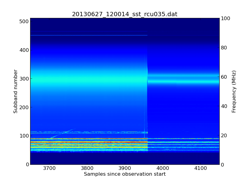 |
| A strange change in the signal level (click to enlarge). |
The above spectrogramme is plotted from a single subband statistics (SST) file. The horizontal axis is time and the vertical axis is frequency. The jet colour scheme shows the log of the received power (dark blue is weak; light blue is stronger).
The transition between the working and failed states took approximately 3 seconds.
We saw the same effect in RCU 034 as well, although here the transition was a bit faster (the data remained good for the first second as RCU 035 was deteriorating and then it changed rapidly to give the same end effect). However, there was no change in any of the other 94 RCU channels.
So, all you LOFAR experts out there... can you tell what caused this abrupt step function in the data?
Subscribe to:
Posts (Atom)