Rescue vehicle at Polaria

Yesterday, on arrival at Polaria for morning coffee, I found a fire engine parked outside the main institute building. No, no fire... just a training course.

Fire engine outside of Polaria (Photo: D. McKay-Bukowski)

Rescue Service, Lapland (D. McKay-Bukowski)

Just to be clear, they were training us about fire safety, not we training them about geophysics. (Although that's an interesting idea...)

KAIRA visual site inspection 5 May 2014

Today I drove up to Tromsø for the quadriphase-coded incoherent scatter radar experiments. As usual, I took the chance to make a visual inspection of the KAIRA site and see how the storm fixes are holding up. In general the site is in a good condition, and, in particular the fixes still look to be well-made! The only thing to be done soon is to collect the styrofoam pieces!

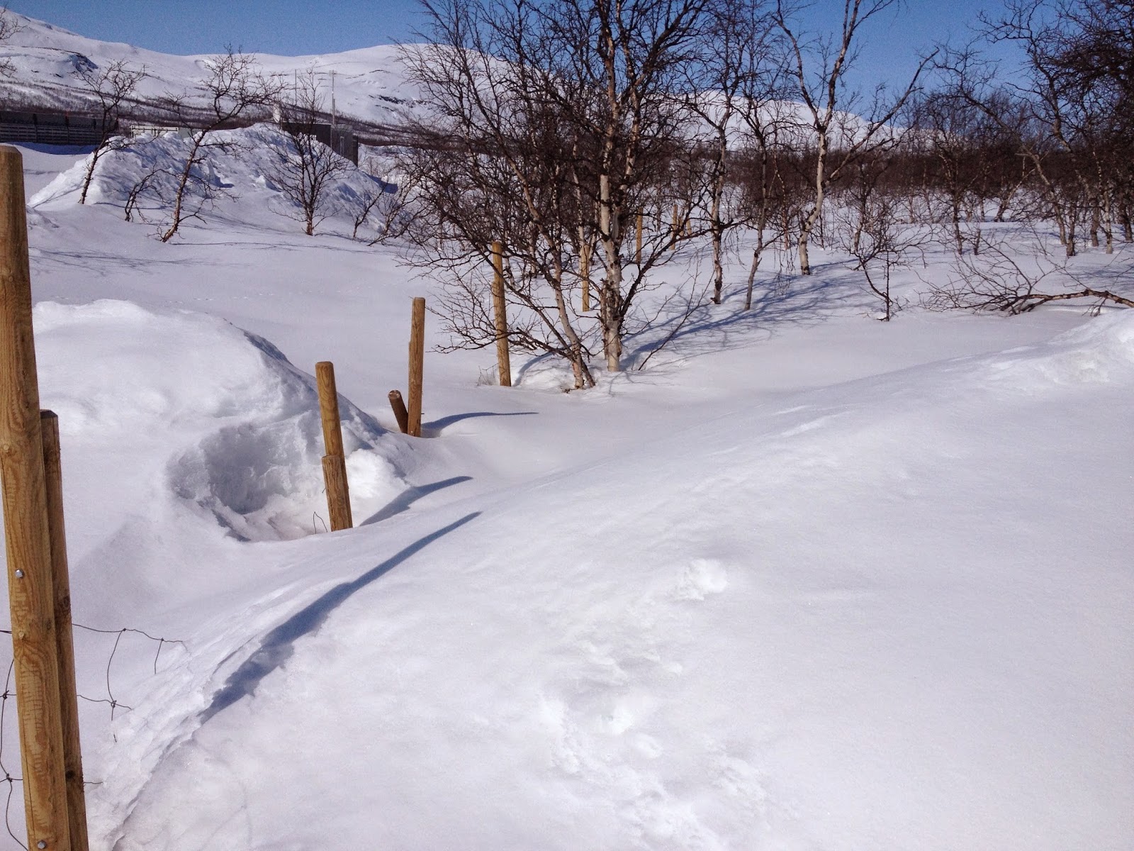
The KAIRA site is inaccessible (without a key), as it is fenced. However, this year in Kilpisjärvi, we have so much snow that one can simply walk to the site (see the first photo)... The snow is really packed, i.e. you do not need even skis!

The reindeer fence next to the main gate is buried by snow!

The site seems to be in a good condition!

One of the snow corridors.

Here is the storm damaged part of the HBA. Fixes are still looking good!

And yep, otherwise the HBA field is in a good condition!

Bits and pieces of the destroyed HBA tile lie around the site.

Emergency fixed LBA antenna! Seems to be a working solution!

Curious ripple in the data

The strange ripple in the dynamic spectrum of the solar radio event from a few weeks back has caught some interest, and we don't have an explanation for it... yet. At first, it was thought it might be an RFI effect, although it is very broad. It also drifts in frequency, which is unusual.

These data are from a single dipole. So, it might be coupling between that and other dipoles, or perhaps Cas A rippling through a sidelobe. For the UK station (which doesn't see the effect -- REF), these sources would be at different position angles. There are several things we have now checked:

We see it on different dipoles. These might have different couplings (due to antenna spacings) or be at different position angles (with respect to, say, a local RFI source).

We also see it on both polarisations. The following two plots are from different polarisations.

LBA aerial #L04, X-polarisation (Image: D. McKay-Bukowski)

LBA aerial #L04, Y-polarisation (Image: D. McKay-Bukowski)

We may still be seeing some sort of ground effect or perhaps a reflection from the reindeer fence. Alternatively, it might be a "snow interferometer" (like the old sea-interferometer, but with a reflection off the snow). The fact is that the sun is at quite a low elevation and the wavelengths are quite long at these frequency bands.

In any case, we remain puzzled. Any suggestions, anyone?

Using median filters in quicklook plots

When we make our plots of spectrum vs. time, we often use a median filter to improve the contrast. The reason for the median filter is that the amplifiers have a certain spectral response associated with them. What you are interested in is the proportional variation of the signal with respect to what it would be if there was no signal.

You can do this by really careful bandpass calibration, but for "quicklook" plots, dividing by the median works and it is very quick. So that's what I use for these plots that I put on the web.

Some subband statistics with a median filter.

The same data, but without the filter.

The Python code fragment looks like this:

        # Determine the median
        med=np.median(data, axis=1)

        # Apply the median to the data
        for i in xrange(data.shape[1]): data[:,i] /= med

Here, "data" is a 2D array with the axes being subband and time.

If you didn't use a median filter, you would expect to see a strong band at about subband 300 (approx. 55-60 MHz). This is due to the peak response of the amplifiers at that region (EXAMPLE). By using the median filter, you remove this bias.


Of course, you still need to be careful. The median filter relies on their being a stable background and more background than signal. In the first plot above, there is a slight negative band around 55-60 MHz, as there was probably a bit too much signal, thus skewing the data. For the purposes of seeing the features, it is not too much of a problem though.
 
The only way to really do this is with a full bandpass calibration but, as mentioned, for a quicklook the median filter gives you a good, easy, high-contrast plot.

EISCAT dish at Sodankylä

Today's Friday Photograph is of the EISCAT dish at the Sodankylä Geophysical Observatory. As you can see, there is still plenty of snow about... even at the beginning of May.

The 32m EISCAT dish at SGO. (Photo: D. McKay-Bukowski)

Have a nice weekend everyone!

Saving and loading data in Python with JSON

Scroll down if you just want to see the example code.

Long-winded pre-amble about computer documentation

If you don't use a computer language too often, then they can be pretty baffling when you come back to them after time away coding up something else. Furthermore, you might find yourself stuck in the mindset (and terminology) of the other language, which makes it pretty difficult to search for the correct terms on the Internet.

Recently, I had just this problem. It was a simple problem.

In Python, I have a record structure (= dictionary) which has labels (= keys) and data (= values). I just want to save it to disk and then later read it back again. That's not so bad, but the one extra point is that I'd like the save file to human-readable, so I can quickly check it with an editor to either see what's there or make corrections.

I quickly decided that "json" was what I needed, instead of  "pickle" (not human-readable files) or csv (seemed to require more work to write out the file). Whether that was the right choice or not is neither here nor there. The fact is that I couldn't quite get it to work.

You see, the json documenation (LINK) while comprehensive doesn't match the terminology I was thinking in my head. Look for the phrase "save to disk" on that page and there is nothing. The word "save" simply does not appear.

Also, if you are used to simple terms like load, save, read, write, etc., then that documentation doesn't read so well. Seriously... go to that page, start at the heading and read it out loud and either listen to yourself and let someone else listen to it. Read to at least the end of the first example.

See what I mean?

Checking websites like StackOverflow finds others occasionally asking similar questions, but with aggressive/arrogant answers along the lines of "the documentation is fine, what's your problem? RTM!"

Well, sometimes we are just on the way to something else. We are scripting, not coding. And we need something in a hurry. We simply don't have the time/skill/experience to get our heads around nested associative array object stream hierarchies (or whatever).

Don't get me wrong. The Python documentation is very good. It is thorough and comprehensive. But if you are coming to it raw and with a problem already in mind, then it can be a bit impenetrable at times. And I have been programming for years and have written many hundreds of thousands of lines of code in various other languages, so I'd hate to think what it would be like for a complete novice.

In any case, if some search engine just happens to put up this weblog post and help one other person in the world who wants a quick and easy, fully working, example of how to write some data to disk and read it back in again, then I'll be happy!   :-)

Saving a Python dictionary to disk using JSON

Okay, here's the code I came up with...

#!/usr/bin/python

# This only uses the json package
import json

# Create a dictionary (a key-value-pair structure in Python)
my_dict = {                   
  'Name':      'KAIRA',
  'Location':  u'Kilpisj\u00E4rvi',
  'Longitude': 20.76,
  'Latitude':  69.07
}

# We can print the dictionary to show we have data. E.g.
print my_dict                 
print my_dict['Location']     

# Open a file for writing
out_file = open("test.json","w")

# Save the dictionary into this file
# (the 'indent=4' is optional, but makes it more readable)
json.dump(my_dict,out_file, indent=4)                                    

# Close the file
out_file.close()

At this point, my little programme has created a file called "test.json". The contents of it look like this...

{
    "Latitude": 69.07, 
    "Name": "KAIRA", 
    "Longitude": 20.76, 
    "Location": "Kilpisj\u00e4rvi"
}

You can edit this as a text file or print it to screen with Linux utilities like 'cat' or 'more'. It can be e-mailed too.

You can tweak the "indent" parameter to change the number of spaces, and there are other options in the json.dump() which can also be used to control the behaviour.

There are some complications if you have non-standard dictionaries or weird data types. You will probably also hit performance issues if you try to save vast quantities of data. However, for the purposes of something quick and simple, this was sufficient for me.

Loading a JSON file into a Python dictionary

Having saved our data, we need to read it back in again. I've done this as a separate programme.

#!/usr/bin/python

# This only uses the json package
import json

# Open the file for reading
in_file = open("test.json","r")

# Load the contents from the file, which creates a new dictionary
new_dict = json.load(in_file)

# Close the file... we don't need it anymore  
in_file.close()

# Print the contents of our freshly loaded dictionary
print new_dict

So, there you go. I hope that helps!

Snow again

Yesterday it started snowing again at Sodankylä... no summer just yet!

Snow at the EISCAT dish at Sodankylä on 29-Apr-2014. (Photo: D. McKay-Bukowski)